As part of recollection, here I gathered some my conceptual analysis on Quantum Mechanics.
1. Preliminary
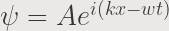
It started when people observed conventional particles, for example, electrons, behave like a wave. This hints a description of particle in wave mechanics, so here we go, we will describe a particle by 
Being a probability amplitude implies that


In other words, the second equation means that particle must be somewhere, we call it normalization condition.
2. Two particles
Now suppose our system has two particles that are sufficiently apart such that there is no interaction between them. The two particles are described by 


It’s not hard to guess that

This really follows from common sense that the probability of two events occurring at same time is the product of the probability of individual event occurring. We could check that it indeed behaves like a probability amplitude.

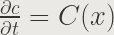
3. Energy conservation
The fact that we could describe a particle by a probability amplitude implies that the information about energy must be somehow encapsulated in the function. This means
![E = E[\psi(x, t)]](https://s0.wp.com/latex.php?latex=E+%3D+E%5B%5Cpsi%28x%2C+t%29%5D&bg=eae9e6&fg=363431&s=3&c=20201002)
Now let’s consider a two-particle system as we described above. We know their energies respectively.
![E_1=E[\psi_1(x_1, t)]](https://s0.wp.com/latex.php?latex=E_1%3DE%5B%5Cpsi_1%28x_1%2C+t%29%5D&bg=eae9e6&fg=363431&s=3&c=20201002)
![E_2=E[\psi_2(x_2, t)]](https://s0.wp.com/latex.php?latex=E_2%3DE%5B%5Cpsi_2%28x_2%2C+t%29%5D&bg=eae9e6&fg=363431&s=3&c=20201002)
The total energy of the system 

On the other hand, if we consider the total probability amplitude of the system, we will have
![E=E[\psi_{12}(x_1, x_2, t)]](https://s0.wp.com/latex.php?latex=E%3DE%5B%5Cpsi_%7B12%7D%28x_1%2C+x_2%2C+t%29%5D&bg=eae9e6&fg=363431&s=3&c=20201002)
By comparison we conclude that
![E[\psi_1(x_1, t)\psi_2(x_2, t)]=E[\psi_1(x_1,t)]+E[\psi_2(x_2, t)]](https://s0.wp.com/latex.php?latex=E%5B%5Cpsi_1%28x_1%2C+t%29%5Cpsi_2%28x_2%2C+t%29%5D%3DE%5B%5Cpsi_1%28x_1%2Ct%29%5D%2BE%5B%5Cpsi_2%28x_2%2C+t%29%5D&bg=eae9e6&fg=363431&s=3&c=20201002)
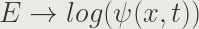
This shows that the form of E must follow a peculiar structure. One familiar function that has the above property is log function.

If this is the case, we would expect
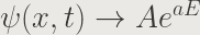
Since there is no justification to say 

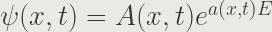
It can’t be right that the probability distribution depends on the energy exponentially. In other words, the exponential dependence must be compensated by an extra term to ensure particle has to exist somewhere, but this obvious contradicts with our assumption that all energy dependence comes in the exponential term. It must be that
where 

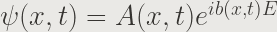
We see that the dependence on 


Now we want to see how

In a closed system, the energy doesn’t change with time, we get

We could infer that the 

The same argument applies that the change of

where 

We could, then, easily figure out the constant
where 

We know the energy of a photon with frequency

Substitute this expression of energy back to the wavefunction
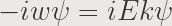


We get the value of

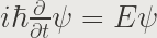
This is in fact one of the very important results in Quantum Mechanics. Through the arguments, one has to conclude that the emergence of complex number is a natural consequence to conserve energy, and in this sense, Quantum Mechanics doesn’t seem that mysterious at all!
