We first define a term called Interest to represent one thing that a person may potentially do. Then we collect all Interests of a person, and organize them in such a way that associated Interests are interconnected. This will give us a huge network of Interests. We then topologically fold our network of Interests into a multidimensional space while keeping connected Interests as adjacent points in space. This space formed is called Interest Space.
Each person is represented as a collection of N Interest points living freely in the Interest Space. We assume each Interest point has equal probability of moving in any direction in the Interest Space. Given N>>1 we can approximate the distribution of Interest points by a continuous function which we call Concentration Function, represented as C(x,t),

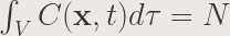
where d is the dimension of Interest Space, and 

Random walk of Interest Point
As the name suggests, the magnitude of Concentration Function will represent the level of concentration at the specific interest point. Our assumption is that each interest point has equal probability of moving in any direction. Anyone with a basic physics training will immediately realize that it reassembles a random walk. For a simplified case where d = 2, it implies a person’s concentration, which is initially at the origin, will move around like shown in Fig. 1. It shows how our concentration will be digressed graphically.

Diffusion of Concentration
When we have a collection of N interest points diffusing simultaneously from the same interest point, from statistics, they follow a Gaussian distribution around the initial interest point, and get flattened through time.

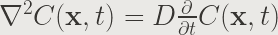
Diffusion Equation of Concentration
An important feature of our construct is the Finiteness of a person’s Interest Points. In other words, we enforce a Conservation of Interest Points. Together with our assumption that each interest point has equal probability to diffuse into its adjacent points, it’s easy to show that our concentration function must follow a continuity equation.
To simplify the problem, we first investigate a one dimensional model. Assuming there is no Boundary Conditions, we can solve the equation with standard separation of variables technique. Given a constraint that C(x,t) must remain real, we get the solution to be like
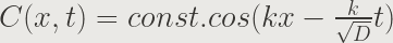
I call this equation Freeworking Equation as we impose no constraints on interest space and time. The implication is that during freeworking, our concentration on any specific interest point will fluctuate sinusoidally with time, and our concentration will fluctuate through related interest points sinusoidally. All these make sense to me.

Importance of boundary conditions
From previous discussion, when there is no constraints, concentration merely fluctuates indefinitely throughout space and time. So here comes the question, how do we raise our concentration on a specific interest point? This is when boundary condition starts to play an important role.
Suppose we have such a constraint that anything outside interest points A and B will be completely ignored. The solutions start to look like in Fig. 4. Compared with our freeworking equation where our concentration merely flows around indefinitely, now they become localized in a certain region. A remarkable fact is that now the solution form a complete set of fourior basics that are able to compose any functions within A and B. Similar effect happens if we constrain our time, we could arbitrarily concentrate on any interest point within A and B.

What does it mean after all?
We have proved that to raise concentration on a specific interest point, we constrain our interest space and time. This is exactly the rationale why we often have to constrain ourselves by setting rigid deadlines and ignore irrelevant topics to be arbitrarily concentrated and therefore achieve great things.
One may ask if we have enough time, why should we care about productivity at all? The ultimate reason is the intrinsic constraint of our lifetime. We simply don’t have enough time. That’s how nature made it to be, neither too short that we can’t achieve anything, nor too long that our concentration starts to diffuse. Nature simply assigns each species an appropriate time scale in preference of productivity. It’s absolutely fascinating!
